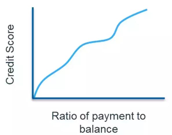
Target encoding, also known as mean encoding or likelihood encoding, is a technique used to convert categorical variables into numerical values based on the target variable in supervised learning tasks. This method is particularly useful in dealing with high cardinality categorical variables (i.e., variables with a large number of unique categories). For credit risk models, this approach is also applied to continuous variables and is popularly known as “Weight of Evidence” (in the context of binary classification problems).

We will derive the above formula, mathematically, for WoE to see where it comes from in the first part of this story. In the second part, we will explore the coding part of it.
The idea is to fit a “piecewise constant” model to the outcome binary variable. This is done by partitioning the variable space into non-overlapping regions such that there is a constant predicted value in each region.
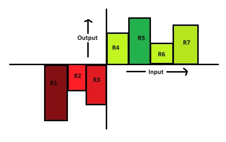
As shown in the figure above, the input space is partitioned into seven non-overlapping regions and the output is a piecewise constant for each region. This is expressed mathematically as follows:

We have a single variable x whose value x_i can belong to a region R_j and we associate a parameter \beta_j with the region R_j. If we have k regions, we get a \beta vector with length k. The piecewise constants will be the estimated values of the parameters \beta_j. Note that the function I is an indicator function which is 1 when x_i belongs to R_j and 0 otherwise.
Before we move further, intuition tells us that if we are fitting a constant value in a region, it should be the “average value” of the outcome in that region. Turns out, that is what we are supposed to get with the following model:
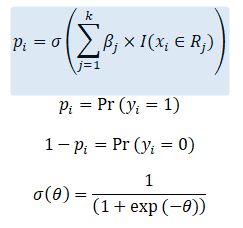
The probability of outcome y_i =1 is given by p_i and is modeled as a function of piecewise constants passed through a logistic or sigmoid function. Note that decision trees work on a similar concept of partitioning of the variable space (they use binary partitions only though).
Also note that Each x_i can be expanded to a vector of dummy variables, i.e., we can convert the input x to k dummy variables:

However, we will avoid dealing with vectors and keep the x_i scalar, and use the indicator function to turn on \beta_j if x_i belongs to R_j. Although we don’t really need the summand before \beta_j we will keep it to formulate the change of j with the region R_j when x_i will fall under R_j.
In general, the above equation for p_i can also be expressed as a function of any x.

Before we move further to derive the WoE values, it is interesting to note that there is no “intercept” term in the above model. Whilst, we could’ve added an intercept term in the above model, turns out that its value will not be defined. The reason is similar to the problem of adding n-values of dummy variables instead of (n-1) values in a regression model, because then intercept can be expressed completely as a sum of all the n-dummy variables, therefore, it is “redundant”. Similarly, here the intercept term is “redundant”. However, it will appear later in the computation of WoE.
We will start by defining the likelihood. Note that y, x, and \beta are vectors and the Likelihood is the joint pmf of y_1, y_2, .. y_n

Now, since we know that If y_i = 1 then P(y_i) = p_i and if y_i = 0 then P(y_i) = 1-p_i, we use it to redefine L

Note: the clever use of the indicator functions which will turn on the specific probability for each y_i. However, we can express this better by using the values y_i themselves.

We can use the above substitution to make our likelihood expression unwieldy:
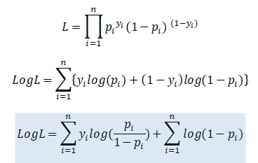
We also take a log of the likelihood because we are working with probabilities and summing them avoids the overflow issues.
Now we substitute our piecewise constant model

And once we do that, we think of the likelihood as a function of the parameter vector because we want to maximize it later on.
We get the following expression for the log-likelihood by substituting values of p_i and also the above expression
 Now comes the main part of maximizing log-likelihood by differentiating it with respect to \beta. For ease, we will partially differentiate it with respect to \beta_j. That is, we want to compute the following partial derivative, and we will do that separately for both the “first term” and the “second term” in the log likelihood expression.

The partial derivative of the first term:

x_i must belong to R_j; only then, we will get the terms associated with \beta_j, whose partial derivative with respect to \beta_j will be 1. Thus, we will be summing over y_i for all those values of i such that x_i belongs to R_j. This is represented by the set I_j. This completes our partial derivative of the first term.

Before we move on to the partial derivative of the second term, we consider the following
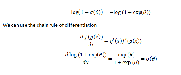
We use the aforementioned concepts and formulae to derive the partial derivative of the second term and we get the following:
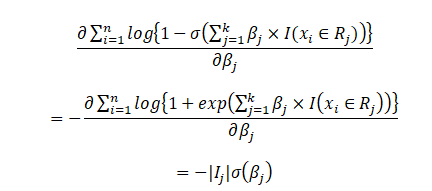
Of course, the “non \beta_j” terms get omitted, even if they are counted over the summand from i=1 to n, while partially differentiating with respect to \beta_j. The lines around I_j indicate the cardinality of the set I_j, i.e., the number of values in I_j.
When we combine the first term and the second term differentials and set it to zero, we replace \beta_j with \hat{\beta_j} because that is the estimate of \beta_j when we maximize the likelihood function.
Thus,

Solving for \beta_j we get.

which are the log-odds for the j-th region R_j
Consider k = 1, i.e., R_1 = {x_1, x_2, …., x_n}

which are the “Overall average” log-odds.
This gives us the value of “weight of evidence” as

WoE is the difference between the log-odds for the j-th region R_j and the “overall average” log-odds. Also, note that instead of using the dummy variable approach, we replace the variable x with is WoE values.


Note: Since there are no restrictions placed on the parameters \beta_j, the regions R_j can have a non-monotonic relationship with respect to the outcome.
