
Authors:
(1) Scott Conn, California Institute of Technology, Pasadena, California;
(2) Joseph Fitzgerald, California Institute of Technology, Pasadena, California;
(3) Jorn Callies, California Institute of Technology, Pasadena, California.
Table of Links
APPENDIX B
YBJ Upper Boundary Condition
Beginning from (A3) with the choice C = 0, we can vertically integrate from 𝑧 = −𝐻 to 𝑧 = 0 and use 𝑀 = 0 at 𝑧 = −𝐻 to arrive at
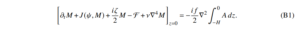
The no-normal flow condition is imposed by requiring ∇𝑀 = 0 at 𝑧 = 0 (Young and Ben Jelloul 1997), which eliminates the advection and dissipation terms. We then horizontally average (denoted by ·) equation (B1). Because 𝑀(𝑥, 𝑦,0,𝑡) has no horizontal structure, it is equal to its horizontal average. On a horizontally periodic domain, all but two terms vanish in the averaged equation:

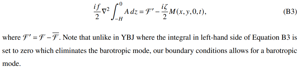
Because the forcing is horizontally uniform in all of our simulations, this reduces to (13). Note that subtracting (B2) from (B1) yields a condition on the integral of 𝐴:
This paper is available on arxiv under CC 4.0 license.